How to scan parameters of DM model with micrOMEGAs.

In this post I show how to scan the parameter space of a BSM dark matter model with micrOMEGAs. If you haven’t set it up yet, download the latest version from its homepage and compile it once

tar -xzf micromegas_6.x.tgz
cd micromegas_6.x
make

If you encounter any installation issue refer to micrOMEGAs manual or README for more details.

Okay, now let us start with a very common task in DM phenomenology, i.e.,

For every DM mass (say $m_{\rm DM}^{}$), find the coupling that reproduces the observed relic abundance, $\Omega h^2 = 0.120 \pm 0.001$.
The resulting curve is the thermal target of the model, and it is the starting point for confronting the model with direct detection, indirect detection and collider bounds.

As a working example I use the simplest DM model there is, the real singlet scalar. micrOMEGAs ships with this model already implemented inside the SingletDM folder, so we can skip model building entirely and focus on the scan.

The model

Take a real scalar $S$ that is a SM singlet and odd under a $\mathbb{Z}_2$ symmetry, $S \to -S$, while all SM fields are even. The scalar potential is

$$\mathcal{V}(S, \Phi) = \underbrace{\frac{\mu_S^2}{2} S^2 +\frac{\lambda_S}{4} S^4}_\text{Dark singlet scalar} + ~\underbrace{\frac{\mu_\Phi^2}{2} \abs{\Phi}^2 + \frac{\lambda_\Phi}{2} \abs{\Phi}^4}_\text{SM Higgs}+ ~\blue{\underbrace{\lambda_{\Phi S} \abs{\Phi}^2 S^2}_\text{Higgs portal}}.$$

	$\text{SU}(3)_c$	$\text{SU}(2)_L$	$\text{U}(1)_Y$	$\mathbb{Z}_2$
$\Phi$	$\mathbf{1}$	$\mathbf{2}$	$+\tfrac{1}{2}$	$+1$
$S$	$\mathbf{1}$	$\mathbf{1}$	$0$	$-1$

Table: Representation of the SM Higgs doublet $\Phi$ and the real singlet $S$.

The $\mathbb{Z}_2$ makes $S$ stable, and the Higgs portal (in blue) is its only link to the SM. After electroweak symmetry breaking the singlet keeps a vanishing vacuum expectation value $\langle S \rangle = 0$ so the $\mathbb{Z}_2$ stays unbroken, while in unitary gauge

$$\Phi = \frac{1}{\sqrt{2}} \pmqty{0 \\ v + h}\,.$$

The masses are then

$$m_h^2 = \lambda_\Phi v^2, \qquad m_{\text{DM}}^2 = \mu_S^2 + \lambda_{\Phi S} v^2 .$$

The portal produces a trilinear vertex $\lambda_{\Phi S}\, v\, h S^2$, which drives both annihilation through an $s$-channel Higgs and scattering off nuclei. The self-coupling $\lambda_S$ plays no role at tree level (I fix $\lambda_S = 0.2$), so the phenomenology is controlled entirely by $(m_{\text{DM}}, \lambda_{\Phi S})$. This is the plane we scan.

The workflow

Each box below is one of the steps that follow.

--- config: block: padding: 18 --- block-beta columns 3 A["1. SingletDM model
parameter names"] space B["2. Relic density
darkOmega"] space:3 E["Results
λ(mDM) curve"] space D["3. Solve for λ
Ωh² = 0.120 ± 0.001"] A --> B B --> D D --> E

1. The SingletDM model

Open your favorite terminal (I like iTerm2!) in the micromegas_6.x/SingletDM directory. The model is defined by the CalcHEP files in work/models/. All we need from them is which variable in the code corresponds to which parameter of the Lagrangian:

Code name	Meaning	Defined in
`Mdm1`	DM mass $m_{\text{DM}}$	`vars1.mdl`
`laSH`	Higgs-portal coupling $\lambda_{\Phi S}$	`vars1.mdl`
`laS`	Dark quartic $\lambda_S$	`vars1.mdl`
`Mh`	Higgs mass $m_h$	`vars1.mdl`
`muSq1`	$\mu_S^2 = m_{\text{DM}}^2 - \lambda_{\Phi S} v^2$ (derived)	`func1.mdl`
`~x1`	The dark scalar $S$	`prtcls1.mdl`

Table: Variables of the SingletDM model.

One thing you should know:

The tilde (~). micrOMEGAs decides which particles are odd under the dark symmetry by their name: anything whose name starts with ~ is treated as dark. That is why the singlet is called ~x1.

Using your own model? Generate the CalcHEP model files (with FeynRules or LanHEP), making sure the dark particles’ names start with ~. Then create a project with ./newProject MyModel, copy the files into MyModel/work/models/, and everything below works the same, apart from the parameter names in assignValW.

I put my own driver (relic.c) directly in the SingletDM directory and compile it with make main=relic.c. You can always play with the provided main.c to check single points. But we want a scan, right?

2. Relic density

The heart of the driver I use is a function that takes $(\lambda_{\Phi S}, m_{\text{DM}})$ and returns $\Omega h^2$:

static double relicDensity(double laSH, double mDM, double *Xf)
{
    int    err, fast = 1;
    double Beps = 1.0e-4;
    char   cdmName[20];

    ForceUG = 1;                /* matrix elements in unitary gauge     */

    assignValW("laSH", laSH);   /* Higgs-portal coupling lambda_{Phi S} */
    assignValW("Mdm1", mDM);    /* DM mass                              */

    err = sortOddParticles(cdmName);   /* recompute spectrum, find the LOP */
    if (err) {
        fprintf(stderr, "Can't compute spectrum: problem with %s\n", cdmName);
        return -1.0;
    }

    double omega = darkOmega(Xf, fast, Beps, &err);
    if (err) fprintf(stderr, "Warning: darkOmega returned err = %d\n", err);
    return omega;
}

assignValW(name, value) sets a parameter by its name in vars1.mdl and warns if the name does not exist. These are the names from the table above.
sortOddParticles must be called after every parameter change. It recomputes the derived parameters and masses and finds the lightest odd particle.
darkOmega solves the Boltzmann equation and returns $\Omega h^2$. It also returns $X_f = m_{\text{DM}}/T_f$, which should be around 20–25 for a WIMP, a useful sanity check. fast = 1 uses the faster approximate integration; Beps controls which coannihilation channels are kept and is irrelevant with a single dark particle.
ForceUG = 1 makes micrOMEGAs compute the matrix elements in unitary gauge. Physical results do not depend on the gauge, but it is a safe habit, and necessary for model files that only implement unitary gauge (it is a global switch, so setting it once at the start of main works just as well).

3. Solving for the coupling

At fixed $m_{\rm DM}^{}$, $\Omega h^2$ decreases monotonically with $\lambda_{\Phi S}$, so finding the right coupling is a one-dimensional root-finding problem,

$$f(\lambda_{\Phi S}) \equiv \Omega h^2(\lambda_{\Phi S}) - 0.120 \simeq 0,$$

and bisection method is the simplest tool for it. Since the required coupling spans about four orders of magnitude over the mass range, it is much better to bisect in $\log\lambda$, i.e. take the geometric mean $\sqrt{\lambda_{\rm lo} \lambda_{\rm hi}}$ as the midpoint:

#define MAX_BISECT 60           /* It seldom needs to bisect this much unless something is wrong!!*/

static int findCoupling(double mDM, double la_lo, double la_hi,
                        double target, double eps,
                        double *laOut, double *omegaOut)
{
    double Xf;
    double f_lo = relicDensity(la_lo, mDM, &Xf) - target;
    double f_hi = relicDensity(la_hi, mDM, &Xf) - target;

    if (f_lo * f_hi > 0.0) return 1;              /* root not bracketed */

    for (int i = 0; i < MAX_BISECT; i++) {
        double la_mid = sqrt(la_lo * la_hi);      /* midpoint in log space */
        double omega  = relicDensity(la_mid, mDM, &Xf);
        double f_mid  = omega - target;

        if (fabs(f_mid) < eps) {                  /* converged */
            *laOut    = la_mid;
            *omegaOut = omega;
            return 0;
        }
        if (f_lo * f_mid < 0.0) { la_hi = la_mid; f_hi = f_mid; }
        else                    { la_lo = la_mid; f_lo = f_mid; }
    }
    return 2;                                     /* no convergence */
}

The scan is then a loop over log-spaced masses, calling findCoupling(mDM, 1e-5, 10.0, 0.120, 1e-3, &laSH, &omega) for each one and writing mDM, laSH, omega to a file (scan.dat below). A tolerance of $10^{-3}$ on $\Omega h^2$ matches the Planck uncertainty, so there is no point going tighter. Write the coupling with %e, not %f: near the resonance it is $\mathcal{O}(10^{-4})$.

Results

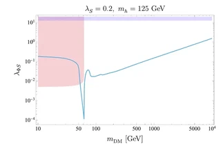
Values of the Higgs portal coupling that give the correct relic abundance as a function of the DM mass.

Figure: Higgs-portal coupling giving $\Omega h^2 = 0.120 \pm 0.001$ as a function of the DM mass, for $\lambda_S = 0.2$ and $m_h = 125$ GeV. The red (purple) region is excluded by invisible Higgs decays (perturbative unitarity).

Every point on the curve gives exactly the observed relic abundance; above(below) it the DM is under-(over-)abundant. If your scan works, you should see three features:

Light DM ($m_{\rm DM}^{}\lesssim 50$ GeV): a nearly flat $\lambda_{\Phi S} \sim 0.1$–$0.2$, from annihilation into $b\bar b$ through an $s$-channel Higgs.
The Higgs resonance ($m_{\rm DM}^{}\approx m_h/2$): a sharp dip down to $\lambda_{\Phi S} \sim 10^{-4}$, because the narrow Higgs enhances the $s$-channel enormously.
Heavy DM ($m_{\rm DM}^{}\gg m_h$): a straight line on the log-log plot, since a fixed $\sigma v \propto \lambda_{\Phi S}^2/m_{\text{DM}}^2$ requires $\lambda_{\Phi S} \propto m_{\text{DM}}$.

Practical tips

Sample the resonance densely. The dip is only a few GeV wide; a 100-point log grid from 10 GeV to 10 TeV puts just a couple of points inside it. Run a separate fine scan over 55–70 GeV and merge.
Flush the output. Call fflush after each point so that a long scan killed halfway keeps what it already computed.

What’s next?

One simple application of the scan is to confront the model with direct detection.

The relic scan is the only step that needs micrOMEGAs. DM-nucleon scattering, $S N \xrightarrow{h} S N $ through a $t$-channel Higgs, involves the same vertex $\lambda_{\Phi S} v\, h S^2$, and at tree level the spin-independent cross section is analytic:

$$\sigma_{\rm el.} \simeq \frac{f_N^2}{\pi} \left(\frac{m_N}{m_h}\right)^4 \frac{\lambda_{\Phi S}^2}{s}, \qquad s = (m_{\text{DM}} + m_N)^2 \simeq m_{\text{DM}}^2,$$

where $f_N \simeq 0.3$ is the Higgs–nucleon coupling. With $m_N \simeq 0.939$ GeV and $m_h = 125$ GeV this gives the handy estimate

$$\sigma_{\rm el.} \simeq 4 \times 10^{-45}~\text{cm}^2 \left(\frac{\lambda_{\Phi S}}{0.1}\right)^2 \left(\frac{300~\text{GeV}}{m_{\text{DM}}}\right)^2 .$$

So once you have the $(m_{\text{DM}}, \lambda_{\Phi S})$ points, a few lines of Python give $\sigma_{\rm el.}$ along the relic curve:

import numpy as np

mDM, laSH, omega = np.loadtxt("scan.dat", unpack=True)   # output of the scan

mN, mh, fN = 0.939, 125.0, 0.30          # GeV, GeV, Higgs-nucleon coupling
GeV2_to_cm2 = 0.3894e-27                 # 1 GeV^-2 in cm^2

s = (mDM + mN)**2                        # s in the non-relativistic limit
sigmaEL = fN**2 / np.pi * (mN / mh)**4 * laSH**2 / s * GeV2_to_cm2

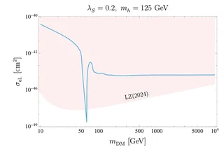
Spin-independent DM-nucleon cross section along the relic density curve, compared with the LZ 2024 limit.

Figure: Spin-independent cross section along the $\Omega h^2 = 0.120 \pm 0.001$ curve. The shaded region is excluded by LZ (2024).

At large mass $\lambda_{\Phi S} \propto m_{\rm DM}$, so $\sigma_{\rm el.}$ is constant, and it sits above the LZ limit all the way to 10 TeV. Only the narrow window on the Higgs resonance survives. This is the generic problem of the minimal Higgs portal.

On a different note, this is one of the reasons why we move to pNGB DM, which can naturally evade these bounds due to its derivative (momentum-dependent) couplings!

Numerical Pheno DM

Authors

Riasat Sheikh

PhD Researcher

I am a PhD researcher in elementary particle theory at Kyushu University, with research interests in dark matter, Higgs physics, and particle phenomenology beyond the Standard Model.

No results found